The Algebra of Coffee Consumption

https://mrhonner.com/2011/06/28/more-clever-accounting/Upon discovering that I had been paying much more for my coffee than I realized, I was faced with a dilemma only algebra could solve.   Or, at least help analyze.

You see, my local coffee shop offers a simple reward program for regular customers:  purchase 10 bags of coffee, and your eleventh bag is free.  At the time of my discovery, I had credit for four bags of coffee.  Thus, the dilemma:  do I continue to buy the over-priced coffee six more times in order to get the free bag?  Or do I just start buying cheaper coffee somewhere else?

The coffee at my local shop was costing me around $12 for 12 ounces.  I knew I could get comparable coffee at another shop for around $10 a pound.  So should I stay or switch?

If I bought 6 more bags from the local shop, I’d spend $72 and get seven 12-ounce bags of coffee (the six I bought, and the free one).  Thus, I would get 84 ounces of coffee for $72.

Now $72 dollars at the new place would get me 7.2 pounds of coffee, or around 115 ounces.  So I’d be getting an additional 31 ounces, or almost two pounds of coffee, by switching!

Needless to say, I swtiched.  But it got me thinking:  at what point would it have been better to continue buying the over-priced coffee?  I turned to algebra for the answer.

Let x = the number of bags of coffee that have already been purchased.  In order to get a free bag of coffee from my local shop, I’d need to buy ten total bags; thus, I’d need to purchase (10 – x) more bags of coffee.  After that, I’d receive one free bag, so in the end I’d get (10 – x + 1) = (11 – x) total bags of coffee.

Each 12-ounce bag of coffee costs $12, so I’d spend a total of $12 * (10 – x) to get (11  – x) * 12 ounces of coffee.

This works out to a price of

\frac{10 - x}{11 - x} dollars per ounce

for the coffee I’d get from the old place.

I know I can get coffee at the other place for $10 per pound, or \frac{10}{16} = \frac{5}{8} dollars per ounce.  Thus, I want to find x so that

\frac{10-x}{11-x} < \frac{5}{8}

which would mean that the coffee from the old place would be cheaper per ounce than the coffee from the new place.

Now we simplify our inequality:

8 * (10 - x) < 5 * (11 - x) ,

\newline 80 - 8x < 55 - 5x ,

25 < 3x,

\frac{25}{3} < x

Thus, I should continue buying coffee at the old place if I’d already bought more than eight bags of coffee there.  Otherwise, I’d be better off switching.

I probably didn’t need algebra to tell me to stick with the old place if I’d already bought 9 bags, but algebra did show me just how hopeless my situation was!

Related Posts

Averia: The Average Font

This is a clever and interesting idea:  creating a new font by taking the average of all existing fonts.

http://iotic.com/averia/

By overlaying all the small letter a‘s, say, from all the different fonts, one can take a visual average and create a new letter a.  Repeat for the whole alphabet, numerals, and punctuation marks, and voila!, you’ve got Averia.

The idea of taking a visual average may be a bit mysterious, but the author describes a few different approaches in how to combine the images.  Essentially all of the instances of a particular symbol are placed on top of each other, and the the darkest parts of the new image are where the instances intersect the most.  The result is then smoothed over to create a readable letter.

And the font looks pretty nice, if not too exciting.  Just what you might expect from the average font.

Disincentive Pricing

While riding the rails around Portugal, I frequently saw passengers buying tickets directly from the conductor on the train.  It got me thinking about how high the penalty should be for not buying your ticket ahead of time.  That is, how much more should you be charged for a ticket purchased on the train than in the station?

You see, if a rider could evade the conductor at a consistent rate, it might make mathematical (if not ethical) sense to gamble on paying the higher fare every so often.  For example, let’s say you can successfully sneak a free ride once every three attempts.  If the ticket in the station costs $5, then the price of the on-board ticket should be at least $7.50 to discourage you from attempting this cheat.

I never found out the price difference in Portugal.  But I do know how it works on the Long Island Rail Road.

Returning from vacation, we were rushing from the airport to the train station.  We didn’t have time to purchase tickets from the machine beforehand as the train was literally pulling into the station as we arrived.  After a long day’s travel, we were happy just to make our connection and get home as quickly as possible.  We figured whatever increase we’d have to pay was worth it.

And it turned out to be nearly a 100% increase.  Instead of the usual $6.25, the on-board charge was $12.  I guess that means they think fare-evaders can get away with it a little less than half the time?

We were happy to get home in a timely manner.  And I was happy to have one more open mathematical question resolved!

Ancient Lego Robotics

The antikythera machine is commonly referred to as the “world’s oldest computer”.  Dating back to around 150 B.C., the mechanism was discovered in a shipwreck around 1900, and it has amazed scientists and engineers with its precision craftsmanship.  Recent x-ray analyses of the object helped bolster the conclusion that it was designed to predict eclipses, and probably was able to do so with remarkable accuracy.

What could be more amazing than a 2000 year old computer?  Perhaps this working replica of it, made entirely out of legos.

https://www.newscientist.com/blogs/nstv/2010/12/worlds-oldest-computer-recreated-in-lego.html

This video shows the functioning lego replica and gives some of the mathematical background relevant to how the machine operates (apparently the ratio 5/19  is extremely important for calculating the cycles of ellipses) .  Throughout the video, the machine is deconsrtucted and you can see the inner-workings of the various parts.  Truly amazing.

NBA Draft Math, Part I

Having put some thought into the mathematics of the NFL draft, I decided to turn my attention to basketball.  From an anecdotal perspective, the NBA draft seems to be more hit-or-miss than the NFL draft:  teams occasionally have success and draft a great player, but it seems more common that a draft pick doesn’t achieve success in the league.

In an attempt to quantify the “success” of an NBA draft pick, I researched some data and ending with choosing a very simple data point:  the total minutes played by the draft pick in their first two seasons.

Total minutes played seems like a reasonable measure of the value a player provides a team:  if a player is on the floor, then that player is providing value, and the more time on the floor, the more value.  I looked only at the first two seasons because rookie contracts are guaranteed for two years; after that, the player could be cut although most are re-signed.  In any event, it creates a standard window in which to compare.

There are plenty of shortcomings of this analysis, but I tried to strike a balance between simplicity and relevance with these choices.

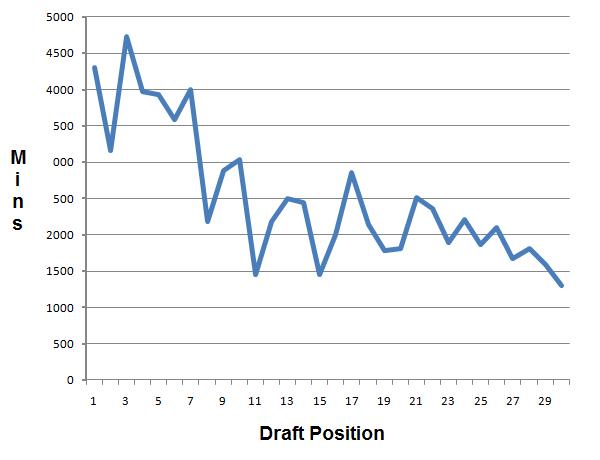
I looked at data from the first round of the NBA draft between 2000 and 2009.  For each pick, I computed their total minutes played in their first two years.  I then found the average total minutes played per pick over those ten drafts.

Not surprisingly, the average total minutes played generally drops as the draft position increases.  If better players are drafted earlier, then they’ll probably play more.  In addition, weaker teams tend to draft higher, and weak teams likely have lots of minutes to give to new players.  A stronger team picks later in the draft, in theory drafts a weaker player, and probably has fewer minutes to offer that player.

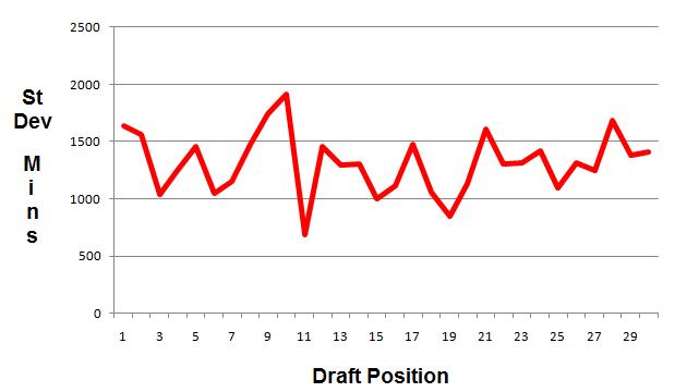
However, when I looked at the standard deviation of the above data, I found something more interesting.  Standard deviation is a measure of dispersion of data:  the higher the deviation, the farther data is from the mean.

Notice that the deviation, although jagged, seems to bounce around a horizontal line.  In short, the deviation doesn’t decrease as the average (above in blue) decreases.

If the total number of minutes played decreases with draft position, we would expect the data to tighten up a bit around that number.  The fact that it isn’t tightening up suggests that there are lots of lower picks who play big minutes for their teams.  This might be an indication that value in the draft, rather than heavily weighted at the top, is distributed more evenly than one might think

This rudimentary analysis has its shortcomings, to be sure, but it does suggest some interesting questions for further investigation.

Related Posts

Follow

Get every new post delivered to your Inbox

Join other followers: