NBA Draft Math, Part I
 Having put some thought into the mathematics of the NFL draft, I decided to turn my attention to basketball. From an anecdotal perspective, the NBA draft seems to be more hit-or-miss than the NFL draft: teams occasionally have success and draft a great player, but it seems more common that a draft pick doesn’t achieve success in the league.
In an attempt to quantify the “success” of an NBA draft pick, I researched some data and ending with choosing a very simple data point: the total minutes played by the draft pick in their first two seasons.
Total minutes played seems like a reasonable measure of the value a player provides a team: if a player is on the floor, then that player is providing value, and the more time on the floor, the more value. I looked only at the first two seasons because rookie contracts are guaranteed for two years; after that, the player could be cut although most are re-signed. In any event, it creates a standard window in which to compare.
There are plenty of shortcomings of this analysis, but I tried to strike a balance between simplicity and relevance with these choices.
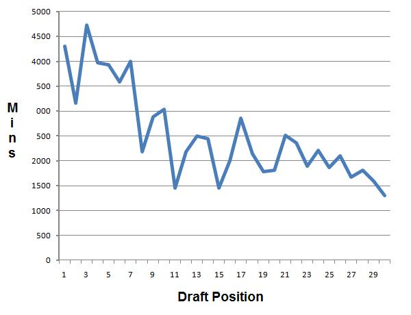
I looked at data from the first round of the NBA draft between 2000 and 2009. For each pick, I computed their total minutes played in their first two years. I then found the average total minutes played per pick over those ten drafts.
Not surprisingly, the average total minutes played generally drops as the draft position increases. If better players are drafted earlier, then they’ll probably play more. In addition, weaker teams tend to draft higher, and weak teams likely have lots of minutes to give to new players. A stronger team picks later in the draft, in theory drafts a weaker player, and probably has fewer minutes to offer that player.
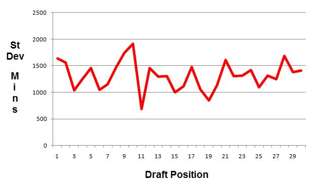
However, when I looked at the standard deviation of the above data, I found something more interesting. Standard deviation is a measure of dispersion of data: the higher the deviation, the farther data is from the mean.
Notice that the deviation, although jagged, seems to bounce around a horizontal line. In short, the deviation doesn’t decrease as the average (above in blue) decreases.
If the total number of minutes played decreases with draft position, we would expect the data to tighten up a bit around that number. The fact that it isn’t tightening up suggests that there are lots of lower picks who play big minutes for their teams. This might be an indication that value in the draft, rather than heavily weighted at the top, is distributed more evenly than one might think
This rudimentary analysis has its shortcomings, to be sure, but it does suggest some interesting questions for further investigation.
Related Posts


5 Comments
Jack "Epic Fail" H · June 21, 2011 at 9:52 am
I really like this concept but the one major issue is someone like Blake Griffin or Greg Oden who spent their whole first years on the bench due to injury, but were not “unsuccessful” players (to whatever degree). Now, you may find that because BG played nearly all of the minutes he possibly could have in year 2 that this evens things out, but it does somewhat obfuscate the reality of the success.
Otherwise, really like this.
MrHonner · June 21, 2011 at 10:37 am
Jack-
It’s definitely a valid point, and one I considered. My goal was to create a very simple, first-pass analysis of the draft, and in doing so I side-stepped the injury issue. Another related issue is the drafting of foreign players who don’t come to play immediately (like Ricky Rubio).
I made the arbitrary decision of looking at the first two years of the contract. Griffin, for example, was under contract during his injury, so I counted the minutes played during his first year as 0. Rubio, on the other hand, was not under contract with Minnesota, so I did not include any data from his pick.
There are certainly many more factors to consider, which is partly why I tried to keep it simple!
PH
Paul Winston · June 26, 2011 at 11:13 pm
Patrick:
Nice analysis.
In a similar vein, I have wanted to model (but haven’t yet gotten around to) the following:
the likelihood of a given team beating another in the NCAAs, as a function of their relative seeds.
I’ve said this about as badly as I possibly could have, but……………………..
if a #2 seed plays a #15 seed, is its likelihood of winning (15/(15+2)) = 15/17, or anywhere close to that number? Is the #15 seed’s win probability 2/17 or (2/17)^2?
As you probably know, no #16 seed has ever beaten a #1 seed in the men’s game, but it has happened a few times in the women’s game.
Any thoughts on this?
Paul W.
Jack "Epic Fail" H · June 27, 2011 at 9:33 am
Hey Paul,
The women’s game would actually be much easier in this regard as there are FAR fewer upsets. Although, as you suggest, the 16 has beaten the 1 seed, the great majority of the time the Final Four in the women’s game is the 1 seeds or close to them so figuring out the formulas for that I imagine would be easier.
As for your model above I think it would have to work out with a less linear relationship as the likelihood of upsets increases greatly as seeds get closer. Furthermore, the reality is that the 1 v 16 game is actually a team seeded 1-4 vs a team seeded 60-64. And if you were to use these numbers in your model, although they are more legitimate, I don’t know that they would work out.
I like this concept though!
MrHonner · June 27, 2011 at 6:38 am
It’s interesting you bring that up, because a student of mine produced a really nice research project on exactly this question. He first looked at seedings as you have suggested, and then generalized to arbitrary weightings for teams and came up with some nice formulas.
I definitely get excited when math and sports intersect.